Understanding the STEPScope®
Time domain reflection and transmission measurements are a convenient way to study signal integrity in high speed systems. Time domain reflection (TDR) enables measurement of impedance mismatches of a DUT which can impact bandwidth and reflections − which can cause bumps in otherwise smooth signals. The TDR measurement shows the impedance of a DUT versus time allowing a diagnostic tool that pinpoints where in the DUT problems might exist. Time domain transmission (TDT) enables seeing what a given DUT will do to a step stimulus as it passes through it. The TDT analysis is a voltage versus time display of the input and output step signals.
What's Inside?
The heart of the STEPScope is a resistively-coupled differential pulser and differential voltage sampler that can both generate fast-edged pulses out the TDR+ and TDR- connectors while simultaneously measuring the signals present at the sampler’s input. A differential resistive summing node is used to achieve the highest signal fidelity by providing a 50-ohm match in all directions. The pulser is a programmable amplitude and frequency square wave which acts as both a stimulus when making reflection measurement into this STEPScope and as a stimulus when making transmission measurements into another STEPScope. Signals that leave the internal pulser outbound to the TDR+/TDR- connectors are attenuated by a factor of 2 by the internal summing node acting as an attenuator.
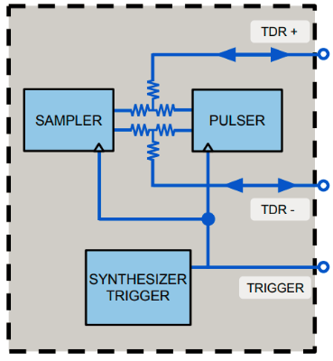 Also inside the STEPScope is a synthesized trigger. This synchronizing trigger is a GHz sine wave. A trigger signal is needed by the sampler to synchronize capture of the voltage waveform. The trigger is also needed by the pulser to know when to generate the fast-edged pulses required. The trigger output can be turned off, making the trigger connector an input. When using two STEPScopes to measure transmission characteristics of a DUT, only one trigger can be active to provide the same triggering synchronization to both STEPScopes. Similarly, when making transmission measurements (where you transmit a pulse from one STEPScope and measure on another) only one pulser can be active and the other must be turned off. A blinking green front panel LED is used to indicate if a STEPScope’s pulser is active. In a measurement setup using multiple STEPScopes, only one STEPScope’s green “Pulser” LED should be blinking.
The sampler will measure a voltage-vs.-time plot of the signal that reaches its inputs. As you can see from the diagram, inputs to the sampler will come from either the TDR+/TDR- connectors or the internal pulser itself. Signals that come from the TDR+/TDR- connectors will suffer a attenuation by a factor of 2 because of the resistive summing node acting as an attenuator. Similarly, signals coming from the internal pulser that reach the sampler will also be attenuated by a factor of 2. The sampler is generic in the sense that it will simply measure the differential voltage vs. time waveform at its inputs. It does not depend on the pulser. If the pulser is turned-off, the sampler will simply measure the signal present at the TDR+/TDR- connectors.
Pulsed signals which leave the pulser and go out to the TDR+/TDR- outputs to a DUT and then reflect part of their energy because of impedance mismatch in the DUT will have the reflected mismatch energy also divided by two on its return trip back to the sampler. This is an attenuation by a factor of four plus the factor caused by the impedance mismatch.
STEPScopes are inherently differential devices. The internal pulser always pulses differentially and the internal sampler always measures a voltage versus time waveform that reflects the difference between its two inputs. STEPScopes can be used in single-ended applications by providing a termination load on the unused TDR- connector and selecting a checkbox in the user interface. This checkbox lets the STEPScope know to scale the results appropriately for a single-ended measurement.
The STEPScope includes two kinds of carefully engineered self-calibration steps. The platform calibrations are used to assure the voltage and time accuracy of all measurements. The platform calibrations consist of noise calibration, a delay calibration, and a flatness calibration. These are executed by pressing the “Calibrations” button on the lower status bar in the user interface. These calibrations take a couple minutes and should be performed once every few months or at the beginning of any critical measurements. The second kind of calibrations are the analysis-specific calibrations. These calibrations include cabling present in the measurement system so that the impact of the cables can be removed. These calibrations must be re-run every time the cabling changes or the temperature of the test system changes. These calibrations consist of attaching 50-ohm loads, SHORTs, or THRUs to the cables and executing the calibration step. Each calibration takes less than a minute to perform.
Reflections
Time domain reflection measurements are based on the physics phenomenon that causes incident energy to reflect back to the source if the impedance of the transmission path changes. The percentage of reflection depends on the ratio of the impedance difference experienced. The sign of the reflection (an inversion of the signal in the time domain) is also set by the impedance difference experienced. We call this coefficient of reflection (the ratio of what incident energy is reflected), gamma. A gamma of 0 means no energy is reflected. This is what happens when our termination perfectly matches our source. A gamma of 1 means all energy is reflected. This is what happens when our termination is an OPEN − we call these signals “inductive”. A gamma of -1 also means all energy is reflected but it is also inverted. This is what happens when our termination is a SHORT. We call these signals “capacitive”.
Transmissions and reflections when a resistive summing node is used have to be carefully considered as the classic responses to typical short/load/open terminations are impacted. To emphasize this point, let’s consider the possible terminations that a STEPScope could see.
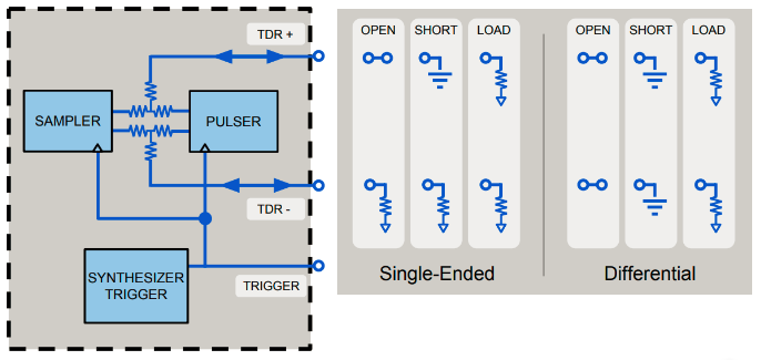
Consider the differential cases first. First, as the pulser transmits its differential output pulse of amplitude A, half of it will go the the sampler directly and the other half will go out the TDR+/TDR- connectors. In this way, the internal sampler will see the same pulse amplitude that the the TDR+/TDR- connectors will see. If we use the default pulser setting of 200mV single-ended signals, each TDR+ or TDR- signal will have a step amplitude of 200mV causing a differential amplitude, A, of 400mV. This would be measured by the internal sampler as the pulse heads to the connectors.
A small time later, the pulse will experience whatever termination we have connected to the TDR+/TDR- connectors. For example, if we sent both our TDR+/TDR- terminations to a 50 ohm load to match the 50 ohm source impedance of the pulser, our reflection coefficient will be 0. No energy will be reflected off the load. In this case, no signal will reverse direction and head back to the sampler so the sampler, which already measured the pulser as it was headed outbound will now continue to hold its final value as no reverse-direction energy will come back to change it. The net effect will be that the sampler measures a single square-wave pulse of amplitude A.
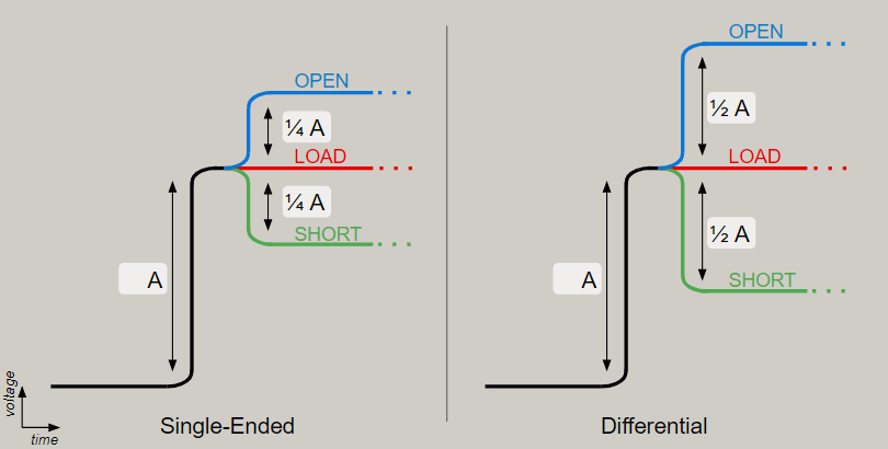 If we change the termination on both TDR+/TDR- to be shorts, our outbound pulse will have a reflection coefficient of -1 on both TDR+ and TDR- legs. This means that all the energy at that point will reverse direction (and reverse sign) and will go back into the STEPScope. As this energy from both legs passes through the resistive summing node inside the STEPScope towards the sampler, it is attenuated by a factor of 2, making it -A/2. The result will be the green “SHORT” waveform.
Similarly, if we change the terminations on both the TDR+/TDR- to be opens, our outbound pulse will experience a reflection coefficient of +1 on both legs. All energy will be reflected, but the sign will not change. Again, this reflected energy will be re-attenuated as it passes through the summing node on the return trip resulting in the blue “OPEN” waveform.
When using single-ended operations, the unused leg is terminated with a 50 ohm load. This makes the maximum reflected energy one-half what it could be if both legs were used. The step response waveform into a 50 ohm single-ended LOAD looks no different; however, the step responses into single-ended SHORT and OPEN terminations have half the reflected energy making their deviations +/- A/4 in this case.
Sampler Voltage Calibration Point (IMPORTANT)
Because of the factor-of-2 attenuation between the three important nodes (the sampler, the pulser, and the TDR+/TDR- connectors) there is a choice of where to reference the displayed voltage on the voltage-vs.-time plot of the sampler. Do you want it calibrated at the pins of the internal sampler? At the pins on the pulser? Or at the TDR+/TDR- connector? For reflection measurements, it does not matter as all measurements are relative. However, for the transmission measurements, it becomes clear that a voltage measurement displayed in a TDT plot would want to be correct with respect to what is presented to the TDR+/TDR- connectors. This, then, presents a problem with respect to measuring the internal pulser’s amplitude. If we calibrate the vertical voltage axis of the sampler including the factor-of-2 attenuation in the path between the sampler and the connectors, and if there is a shared factor-of-2 attenuation for the pulser to both the sampler and the connectors, then we end up interpreting the internal pulser amplitude as two times the amplitude of the pulser at the connector.
When measuring the internal pulser’s amplitude on the internal sampler, the amplitude is twice what it will be at the TDR+/TDR- connectors. An internal pulser setting of 200mV single-ended will create a differential pulse that is 400mV, and the internal sampler will measure it as 800mV.
Pulser Settings
Large pulser amplitudes may damage semiconductor circuits, so the default pulser amplitude is set to a low 200 mVse. If the pulser amplitude is increased, more energy can be reflected making it easier to measure in face of noise in the measurement system. In passive systems, larger amplitudes can easily be used.
Shorter pulse widths can also be set on the STEPScope. This allows more pulses per second which decreases measurement time. However, if pulse widths become too short, reflected energy may not have died out from one pulse in time for the next pulse and would then pollute the next measurement. This can depend both on the electrical length of the circuit under test as well as the extremes of the impedance mismatch. The default setting for pulser width is a good compromise for quick measurements over long times. Applications in very fast production testing might adjust these numbers specific to their use case.
Analysis
A pulser-sampler combination such as this can be used for many things including reflection and transmission measurements. Reflection measurements are measurements of reflected energy in response to a forward stimulus. For example, when a STEPScope’s pulser sends a fast pulse into a DUT and the reflected energy comes back to the STEPScope it is measured. Because the STEPScope has calibrations for what reflects from good loads and perfect shorts, it can separate-out the reflected energy from the transmitted energy. This ratio of transmitted to reflected energy is the gamma which can be properly scaled to measure the impedance versus time familiar to a Time Domain Reflection (TDR) measurement.
Similarly, by using two STEPScopes, it is possible to have one STEPScope send a fast pulse into a DUT and image the response to that fast pulse using another STEPScope’s sampler. By first making a calibration measurement without the DUT in the path, a direct comparison of with-DUT and without-DUT can be made. For example, if a fast pulse edge measured in the “without-DUT” case is slowed-down in the “with-DUT” case, and estimate of the DUT bandwidth can be made. This type of measurement is called “Time Domain Transmission (TDT)” and results in a voltage-vs-time display.
Time Domain Reflection (TDR)
TDR analysis uses the measured step responses of a DUT along with previously-taken calibration step responses to compute the ratio of incident and reflected waveforms and scale them to ohms. All this is done versus time to present a graph of ohms versus time. Time, in this graph, is two times the one-way delay into the DUT because reflected measurements necessarily require a round-trip (two times) delay to make a measurement. Calibration waveforms capture the response to a step with a 50-ohm load as well as with a SHORT. The response to the 50-ohm load, where no energy is reflected, is used to define a zero-reflection response and to remove noise. The response to a short, where all incident energy is reflected (and inverted) and sent back to the STEPScope, is used to determine the incident waveshape. When using single-ended operation, calibration terminations are applied to the single-ended leg you are using (and a 50-ohm load is left connected to the other TDR connector). When using differential operation, both legs (TDR+ and TDR-) must have the prescribed calibration load connected.
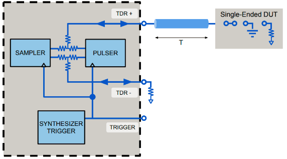 TDR measurements on a single STEPScope can be made in either single-ended or differential applications. In either case, typically, one or two cables are added to the front of the STEPScope to make it convenient to connect to a DUT. Customers often don’t want to include this cable in their measurement so they want to “move their reference plane” to the end of the cable(s). This is done by calibrating the TDR with the cable(s) connected. This delays the incident wave’s arrival to the DUT by T as well as any reflected wave’s return-path arrival to the STEPScope’s sampler by another T, but these delays to not impact the TDR measurement. Long or poor cables can impact the bandwidth of the measurement and would also be a reason to use a longer pulse width to allow more settle time to separate one measurement from the next.
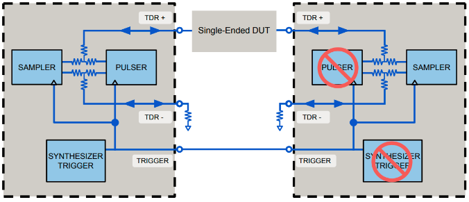
This figure shows the single-ended configuration. Note the termination on the front panel TDR- connector. The principal of moving the reference plane holds for either single-ended or differential configurations. When using differential configurations, matched-length cables must be used.
Time Domain Transmission (TDT)
Active and passive DUTs such as cables, backplanes and amplifiers will change a signal as it passes through it. These changes may be due to resistive losses of the conductor, dielectric losses in the medium, impedance inflections due to mechanical configurations, etc. Observing what a DUT will do to a fast-edged pulse is the job of TDT. When using TDT, two STEPScopes are required. One is the pulser and the other is the sampler. It is not possible to use the pulser and sampler from one STEPScope for this configuration.
 When using two STEPScopes, it is important to share the “Trigger” signal between both units. This can be done by connecting an SMA cable between the two “Trigger” connectors. This connection is a GHz sine wave so it is very insensitive to the quality and length of this cable. When more than two STEPScopes are needed, a splitter (and even an amplifier) can be used to make enough copies of this signal to connect to all STEPScopes in the system.
Also when using more than one STEPScope, it is very important to only enable one Pulser. All other STEPScope’s pulsers must be turned off. The green Pulser LED on the front panel will blink when a STEPScope’s pulser is active. Only one STEPScope’s pulser should be blinking at a time. When configured to make a TDT measurement into a second STEPScope, it is also possible to simultaneously make a TDR measurement into the first STEPScope.
During TDT calibration, a reference waveform is captured with the DUT removed. Typically, a small high-quality barrel connector is put in its place during the calibration measurement. This measured reference waveform represents the incident wave presented to the DUT. It defines the both the waveshape (amplitude, risetime, etc.) and the phase. Once the DUT is re-inserted in the measurement path, the measured response will show the transmitted waveform. TDT can be displayed in two ways − with and without forced phase alignment. The through-calibration reference waveform edge is always positioned at time zero. When displaying the TDT waveform without forced phase alignment, the TDT waveform will represent the true delay between the reference and TDT signal arrival caused by the extra length of the DUT. This makes it easy to measure the added DUT delay. When displaying the TDT waveform with forced alignments, the TDT DUT waveform is purposely overlaid on top of the calibration reference waveform to make it easier to compare edges.
The “through” calibration for TDT must be made anytime the cabling changes or the trigger source or synthesizer source is changed. An interruption of the trigger will cause a synchronization loss between the two STEPScopes which means a new “through” calibration is needed to regain phase.
Both calibration reference waveforms and DUT TDT waveforms can be exported to .CSV files in either their “aligned” or “not-aligned” form. This makes it easy to process these waveforms with other tools, including comparing their spectrums to find the insertion loss spectrum of the DUT.
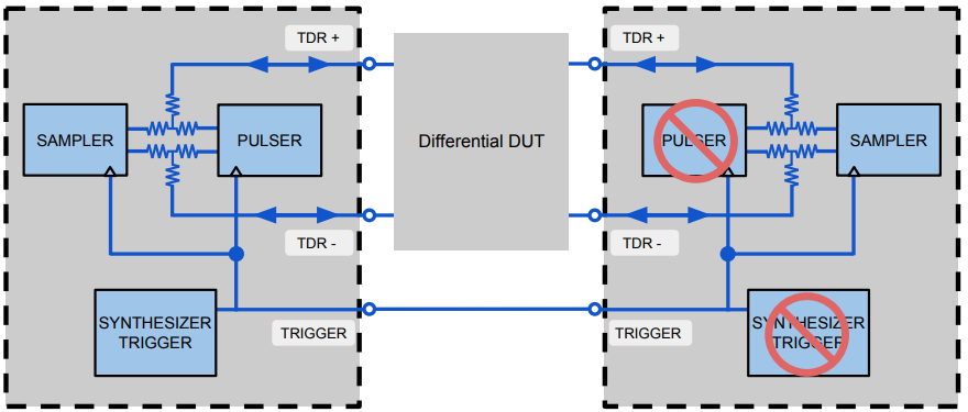
Differential TDT works exactly the same way. In the differential case, both TDR+ and TDR- connections must be made. During through-calibration, two high-performance barrel connectors must be used along with matched cables.
Terminations for Calibration
Finally, a note about the quality level of terminations (not supplied) used during calibration steps. There is a wide range of quality versus price in screw-on terminators (both shorts and loads). A high-quality termination is characterized by a very sharp (high bandwidth, broadband bandwidth) transition as seen in a reflection or through measurement as well as precise 50-ohm values. At high bandwidths, even economy kits that include differential terminations for male and female versions of these devices can cost as much as a STEPScope. For this reason, it is important to understand the impact of using lower-quality termination loads during calibration steps in the STEPScope.
During platform calibrations some of the steps require attaching 50-ohm loads to the TDR+ and TDR- connectors. During these tests, there is no requirement for precision here. A low-cost 50-ohm terminator can easily be used.
During TDR calibrations it's a different story. A low-cost SHORT termination will not have as clean and as fast a transition when reflecting incident energy. Therefore, the captured step response will have a slower and disturbed edge at the beginning of the step. This can influence the accuracy of any ohm measurement made during the few picoseconds near the transition. However, it won’t impact the accuracy of ohms measurements made later on in the response.
When a low-cost LOAD termination is used, there are two potential impacts. First, the transition into the load can be disturbed with momentary inductances or capacitances inside the terminator. This is typically short in duration and, again, occurs only around the time where the terminator is applied. This would mean that an ohms measurement made in a DUT right near the beginning of the DUT (near the same physical lengths of where the low-cost terminator was used during calibration) could be suspect.
The second impact of a low-cost LOAD is that the DC termination resistance is often not 50 ohms. It is very typical for low-cost terminators to range from 48-52 ohms. For this reason, the STEPScope allows input of the actual ohms used during calibration which will offset the TDR results. This value can be checked with an ohm meter. Day to day, routine TDR measurements providing critical insight into signal integrity can be made with good accuracy using low-cost termination.
Frequently Asked Questions
How do I find my IP address?
There are a few options, check out the guide here.
Is the information stored on my BitWise device secure and private?
Yes. There is no centralized server that connects to each device and gathers acquired data, processes it, and provides results back to the user-interface site and to the user. All the acquisition and processing is done inside each device, and the browser-based graphical user interface comes directly from inside the device itself. The device is normally connected to the customer's local area network so that it may provide the user interface site to users inside the local area network. When the device is turned on, it asks the local area network to assign it a local IP address using standard DHCP protocols (just like any other computer on the local area network). Then, a computer on the local area network can access the user interface by opening a browser and pointing it to the IP address of the device. Nothing about this setup utilizes the internet − only your local area network. To demonstrate this, one could connect the device and a laptop to an inexpensive router that supplies DHCP and DO NOT CONNECT the router to the internet. In this configuration, the device will operate normally and enable the computer to direct its browser to the user interface supplied by the device.
There is one feature that does use the internet, called "Lookup local device IP address." This is a convenience feature to assist in finding the local IP address for the device on the local area network. This feature is operated by accessing an INTERNET website www.bitwiselabs.com. The website asks the user to press the button on the back of the device, which causes the unit to attempt to reach the internet and transmit three pieces of information: 1.) The type of device, 2.) The serial number such as "000009", and 3.) the local area network IP address for the device. Notice this is a local area network IP address which cannot be used outside the local area network. The website asks the user to enter the serial number, and it provides a link on the website page that will only be resolved if it is accessed from inside the same local area network as the device.
What is the thick hashed line on the TDR display?
The Calibration step acquires a portion of the pulse based on locating where the reference plane exists based on detecting waveform transitions in the acquired data. Subsequently, this data is interrogated during running mode to calculate the TDR display in conjunction with the newly acquired data at the current pan and zoom levels of the chart. If you pan or zoom outside the range of the calibration data, then no reference is available and this is indicated by the thick, hashed line on the display.
What are we calibrating when we do a TDR calibration?
Calibration waveforms capture the response to a step with a 50-ohm load as well as with a SHORT. The response to the 50-ohm load, where no energy is reflected, is used to define a zero-reflection response and to remove noise. The response to a short, where all incident energy is reflected (and inverted) and sent back to the STEPScope, is used to determine the incident waveshape. When using single-ended operation, calibration terminations are applied to the single-ended leg you are using (and a 50-ohm load is left connected to the other TDR connector). When using differential operation, both legs (TDR+ and TDR-) must have the prescribed calibration load connected. Some tests will require high-end termination calibration kits, but most will make due with inexpensive kits. Read more here.
What are we calibrating when we do a TDT calibration?
TDT Calibration is needed to measure the "BEFORE" waveform in a TDT analysis. BEFORE waveforms are considered the reference waveform and can be displayed on the voltage versus time display along with the DUT's "AFTER" waveform for comparison. For example, comparing the rise-time of the BEFORE waveform to the rise-time of the AFTER waveform can be used to quickly estimate channel bandwidth.
What is being displayed on the TDT graph?
The TDT graph is a voltage versus time display of the measured waveform along with the voltage versus time display of a "through" reference waveform. This shows what the waveform looks like BEFORE and AFTER it has passed through a DUT (e.g. channel).
Can I measure delay of the inserted channel by using the TDT cursors?
Yes, as long as the "Line-Up Reference Edge" is not selected. After a new "through" calibration to establish the phase of the reference edge, the DUT (e.g., channel) waveform will be drawn with the delay that was seen when the waveform was measured. The X-cursors can be used to measure this difference.
How often are "platform" calibrations required? What does this depend on?
Platform calibration should be performed when first using the STEPScope, then every couple of months, or before sensitive tests.
When/Why do we set the pulser width to a specific value?
The shorter pulser widths will make taking measurements faster. However, if the electrical system being tested is too long, then short pulse widths will interfere with each other before they can die out in the system.
What does the flashing light on the front mean?
The "Pulser" LED indicates if the pulser inside is enabled. In certain cases (e.g., TDT) a pulser from one StepScope is driving the input of another StepScope. In this case, only the "Pulser" LED on the pulse-driving StepScope will be blinking.